Study Notes - Artificial Intelligence (AI) and Machine Learning (ML)

29 Jun 2018 • 11 min. read

These are my raw personal notes covering common concepts and techniques.

Some caveats:

• This post may not be helpful for your purposes.
• This is still very much a work in progress and it will be changing a lot.
• Some content may be out of order, missing. Don’t get upset.
• The notes are created in (GitHub flavored) markdown, so unfortunately lack snazzy interactivity.
• Part of this material is adapted, sometimes directly copied from elsewhere.

Should you find grave errors, let me know.

---

Table of Contents

1. What is Machine Learning?
   • 1.1 Functions
   • 1.2 Algorithms - Grouped by Learning Style
   • 1.3 Supervised v. Unsupervised
2. Techniques
   • 2.1 Regression
   • 2.2 Classification

---

1. What is Machine Learning?

Machine learning provides the foundation for artificial intelligence. We train our software model using data e.g. the model learns from the training cases and then we use the trained model to make predictions for new data cases.

Let’s start with a data set that contains historical records aka observations. Every record includes numerical features (X) quantifying characteristics of the item we are working with.

There are also values we try to predict (Y). We will use training cases to train the machine learning model so that it calculates a value for (Y), from the features in (X). Simply said, we are creating a function that operates on a set of features, (X), to produce predictions, (Y): f: X → Y.

1.1 Functions

At heart, a function is the mapping from a set in a domain to a set in a codomain. A function can map a set to itself. For example, f(x) = x2, also notated f: x ↦ x2, is the mapping of all real numbers to all real numbers, or f: R → R.

The range is the subset of the codomain which the function maps to.

Functions don’t necessarily map to every value in the codomain. Where they do, the range equals the codomain.

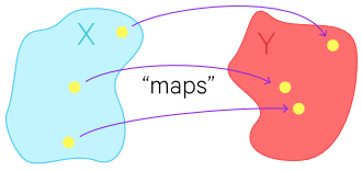
There are 2 sorts of functions. Functions which map to R, are known as scalar-valued or real-valued. Functions which map to Rn where n > 1 are known as vector-valued.

Ref: Web: Mathworld Wolfram - Eric W. Weisstein.

1.2 Algorithms - Grouped by Learning Style

• Supervised learning - the algorithm is given a pre-labeled training example to learn from.
• Unsupervised learning - the algorithm is given unlabeled examples.
• Semi-supervised learning - the algorithm uses a mix of labeled & unlabeled data.
• Active learning - similar to semi-supervised learning, but the algorithm can “ask” for extra labeled data based on what it needs to improve on.
• Reinforcement learning - actions are taken and rewarded, or penalized; goal is maximizing lifetime/long-term reward (or vice versa).

Ref: Book: Neural Computing: Theory and Practice (1989) - Philip D. Wasserman.

Note: Following course guidelines, we’ll discuss the two most common methods; supervised and unsupervised.

1.3 Supervised v. Unsupervised

In a supervised learning scenario, we start with observations that include known values for the variable we want to predict. We call these labels.

Because we are starting with data that includes the label we are trying to predict, we can train the model using only some data and hold the rest for evaluating our models performance.

We’ll then use a algorithm to train a model that fits features to the known label.

As we started with a known label value, we can validate the model by comparing the value predicted by the function to the actual label value that we knew. Then, when we’re happy that the model works, we can use it with new observations for which the label is unknown, and generate new predicted values.

Typical notation:

• m = number training of examples
• x’s = input variables or features
• y’s = output variables or the “target” variable
• (x(i), y(i)) = the ith training example
• h = hypothesis i.e. the function that the algorithm learns, taking x’s as input and outputting y’s

In a unsupervised learning scenario, we don’t have any known label values in our training data set.

We’ll train the model by finding similarities between observations. Once we have trained this model, more observations are added to a cluster of observations with alike characteristics. (Cluster = Group)

2. Techniques

2.1 Regression

When we need to predict continuous valued output (i.e. a numeric value), we use a supervised learning technique called regression.

Let’s take one male. We want to model the calories burned while exercising.

First we get some pre-liminary data (age: 34, gender: 1, weight: 60, height: 165), then put him on a fitness monitor and capture additional information. Now what we do is model the calories burned using features from his exercise like his heart rate: 134, temperature: 37, and duration: 25.

In this case we know all features and have a known label value of 231 calories. So we need our algorithm to learn a function, that operates of all the males exercise features to give us a net result of 231.

• f([34, 1, 60, 165, 134, 37, 25]) = 231

A sample of one person isn’t likely to give a function that generalizes well. So we gather the same data from a large number participants, and then train the model using the bigger set of data.

• f([X1, X2, X3, X4, X5, X6, X7]) = Y

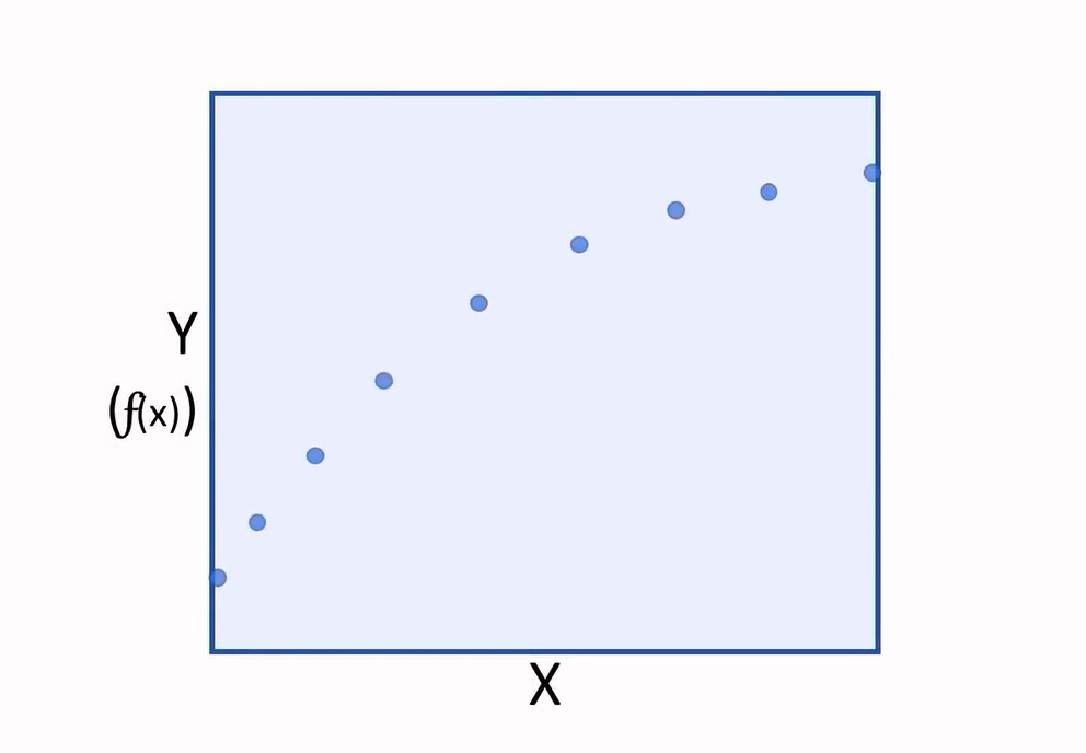
Now having a new function that can be used to calculate label (Y), we can finally plot the values of (Y) calculated for specific features of (X) values, on a chart:

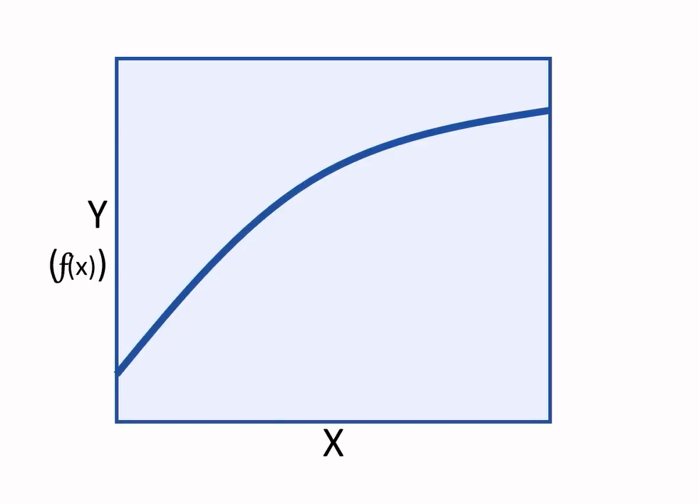And we can interpolate any new values of (X) to predict an unknown (Y).

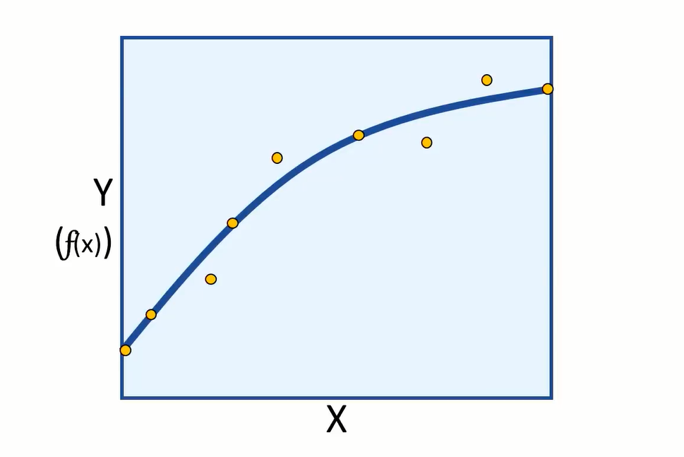
As we started with data that includes the label we try to predict, we can train the model using some data and keep the rest for evaluating the models performance. Then we can use the model to predict (F) of (X) for evaluation data, and compare the predictions or scored labels to the actual labels that we know to be true.

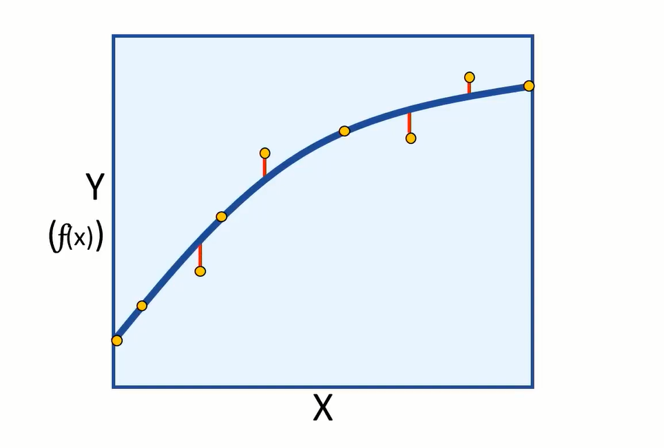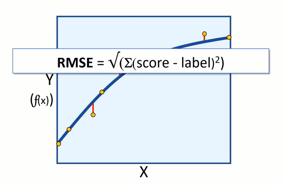
The difference between the predicted and actual levels are called the residuals. And they can tell us something about the error level in the model.

We can measure the error in the model using root-mean-square error or (RMSE) and mean absolute error (MAE).

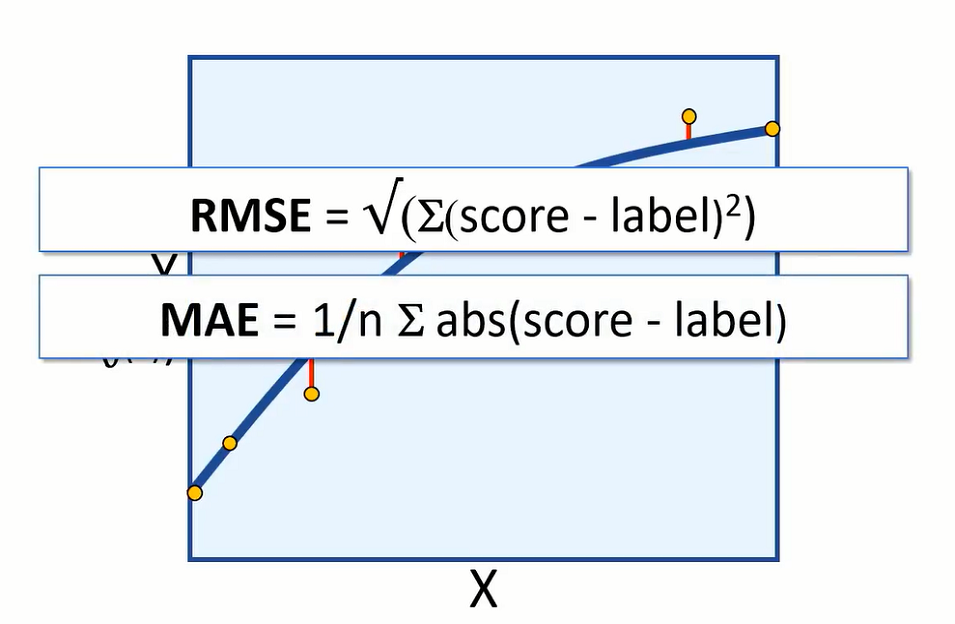Both are absolute measures of error in the model. For example, having an RMSE value of 5 would mean that the standard deviation of error from our test error is 5 calories. An error of 5 calories seems to indicate a reasonably good model, but let’s suppose we are predicting how long an exercise session takes. An error of 5 hours would be a very bad model.

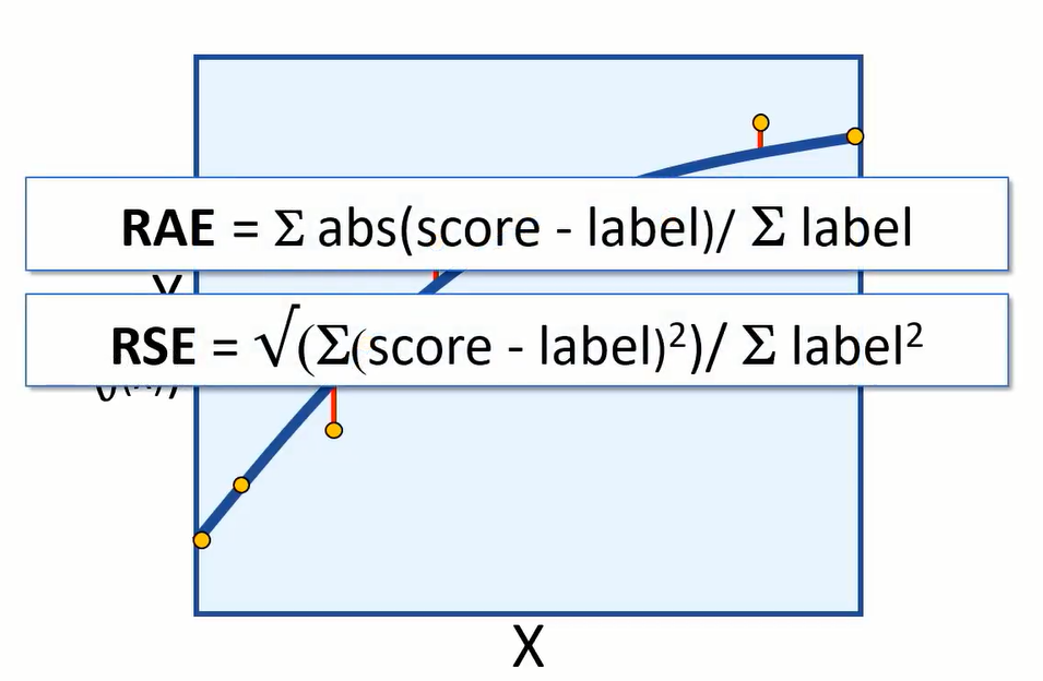
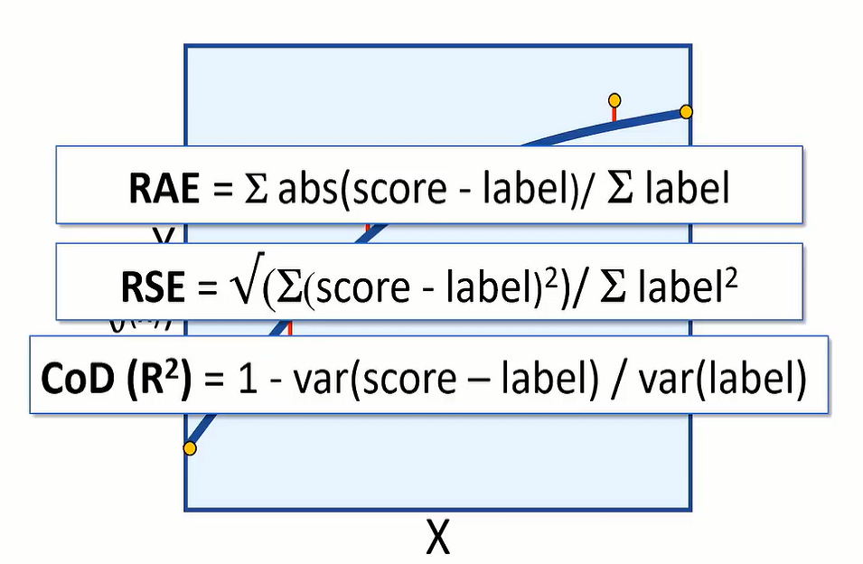
You might want to evaluate the model using relative metrics, to indicate a more general level of error as a ‘relative value’ between 0 and 1. Relative absolute error (RAE) and relative squared error (RSE) produce metrics where the closer to 0 the error, the better the model.

Coefficient of determination (CoDR) or R squared, is another relative metric, but this time a value closer to 1 indicates a good fit for the model.

2.2 Classification

Another kind of supervised learning is called classification.

Classification is the technique that we can use to predict which class or category something belongs to. A simple variant is binary classification, where we predict whether entities belong to one of two classes (true or false).

Example, we’ll take a number of patients in a health clinic, gather some personal details e.g. age: 23, pregnancy: 1, glucose: 171, BMI: 43.5, run tests, and identify which patients are diabetic and which are not.

We could learn a function that can be applied to the patient features and give us the result 1 for patients that are diabetic:

• f([23, 1, 171, 43.5]) = 1

and 0 for patients that aren’t.

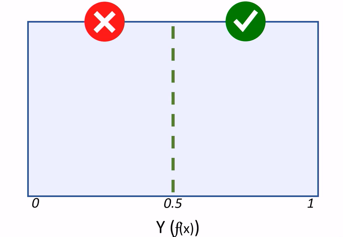
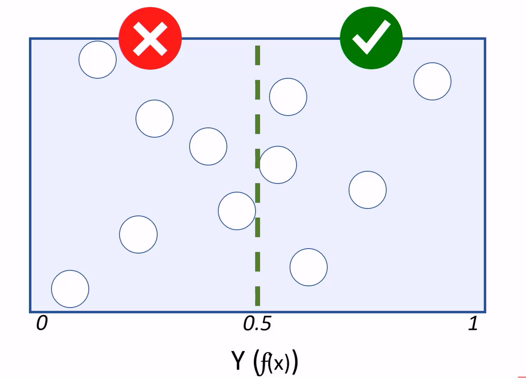
Generally, a binary classifier is a function, that can be applied to features (X), to produce a (Y) value of 1 or 0. This function won’t actually calculate the absolute value of 1 or 0. Instead it calculates a value between 1 and 0: Y(f(x)) and we’ll use a threshold value to decide whether the result should be counted as 1 or 0.

When using this model to predict values, the resulting value is classed as 1 or 0, depending on which side of the threshold line it falls.

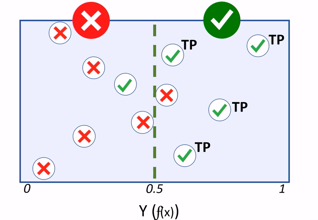
Because classification is a supervised learning technique, we withhold some of the test data to validate the model using known labels.

Cases where the model predicts a 1 for a test observation, while holding a label value of 1, are considered true positives.

Cases where the model predicts 0, and the actual label is 0, are true negatives.

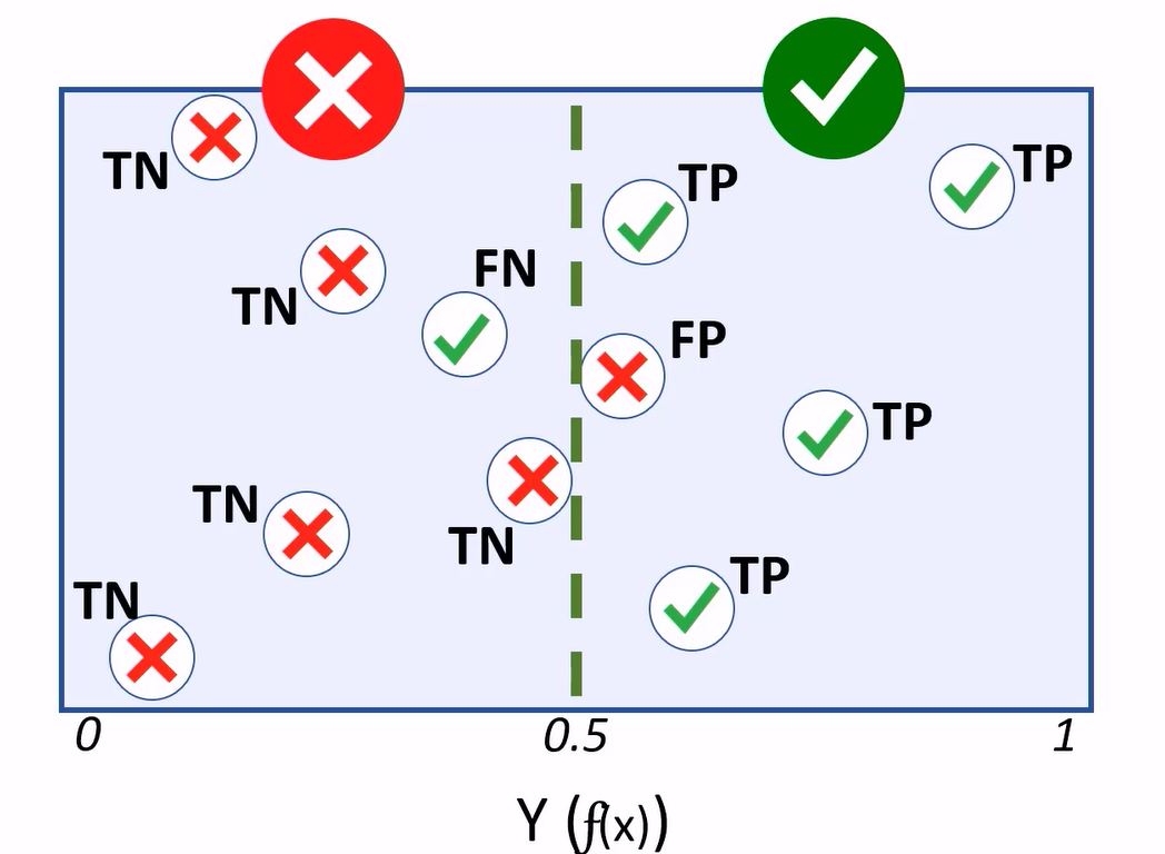If the model predicts 1, but the actual label is a 0, that’s a false positive.

If the model predicts 0, but the value is 1, we have a false negative.

A treshold determines how the predicted values are classified. For your diabetes model, having more false positives, thus reducing the amount of false negatives, will be better as more people with a risk of diabetes get identified.

The total number of positives and negatives generated by a model are crucial in evaluating its effectiveness. For that purpose we’ll use this confusion matrix e.g. our basis for calculating performance metrics for the classifier.

Ref: Web: MSXDAT262017 - edX.

9. In Practice

Before you start building your machine learning system, you should:

• Be explicit about the problem.
• Start with a specific question. What do you want to predict, what tools you have to predict it with?
• Brainstorm on possible strategies like what features might be useful, or do you need to collect more data?
• Try and find good input data.
• Randomly split data into: training samples, testing samples and validation samples.
• Use features of, or features built from the data, that may help with making predictions.

To start:

• Start with a simple algorithm which can be implemented quickly.
• Test the simple algorithm on your validation data, evaluate the results.
• Plot learning curves to decide where things need work. As example, do you need more data, features?
• Analysis: manually examine examples in the validation set your algorithm made errors on.

To generate a learning curve, you deliberately shrink the size of the training set and see how training and validation errors will change as you increase the size.

With smaller training sets, we expect the training error will be low because it is easier to fit to less data. As the training set size grows, your average training set error is expected to grow. Conversely, we expect the average validation error to decrease as the training set size increases.

If the training and validation error curves flatten out at a high error as set sizes increase, then you have a high bias problem. Adding more training data will not (by itself) help much.

On the other hand, high variance problems are indicated by a large gap between training and validation error curves as training set sizes increase. You would see a low training error. In this case curves are converging and adding data helps.

Ref: Web: Intro to Artificial Intelligence - Udacity.