21 Aug 2020 •
2 min. read
Hey, what do you mean with “Docs-as-Code”?
The concept “Docs-as-Code” is basically similar to the way software engineers:
- Write code,
- Build an executable,
- Test it, and then publish the deliverable.
In technical writing terms, it can look something like:
- Store your content source in a version control system like GitHub (typically in a format like Markdown),
- Using static site generators like Middleman, Gatsby, Hugo, Jekyll, VuePress, MKDocs etc.,
- Produce a documentation site, running some validation checks (like broken links) and then publish it to your hosting provider.
Should I treat documentation the same as my source files?
Source code and documentation files (even if written in MD) are not the same.
A source code file is in plain text. A compiler reads the file and converts it into a machine-readable format (like an executable file).
A documentation file on the other hand will require extra elements, such as:
- A link to an image (where will it be hosted),
- Who is going to upload what,
- Different rich styles like Tables, Tabs, Source code viewer, etc.
In terms of source code files, compilers are pretty mature and stable. If there are syntax errors (not functional errors) the compiler will catch them immediately.
Converting Markdown (using a static code generator parser) to HTML is prone to errors. There is no defined syntax for formats like MD, merely various flavours.
Challenges encountered when using this approach:
- Simple fixes are complex,
- Editorial workflow and review processes,
- Image management and preview,
- Category management,
- Search implementation,
- When devs need to write technical docs, things can go frantic.
Is it worth the trouble?
Docs differ significantly when compared to source code. In theory, it might look fascinating to go down the “Docs-as-Code” path.
In practice it can get quite rough, especially when you’re this single guy creating software documentation in a few GitHub repos, or writing some technical posts. If that’s the case, I suggest skipping or you should like self-punishment.
Big companies with dedicated teams should look at tools like docToolChain. The philosophy of docToolchain is that software documentation should be treated in the same way as code together with the arc42 template for software architecture.
Further reading (English books)
19 Mar 2019 •
5 min. read

These notes are meant to help you setup a dual-booting system on a computer running Windows 10 Professional using BitLocker Device Encryption, Modern Standby (a.k.a. Fast Boot), and Secure Boot.
Linux installation is covered briefly as we will focus on preserving the Windows pre-boot UEFI environment in such a setup.
MAKING PREPARATIONS
Before proceeding you should backup all important data to an external disk or your preferred online backup provider. Remember… there is a not insignificant risk of permanently breaking the Windows 10 installation in a non-recoverable fashion as you’ll be making changes to the UEFI partition in your computer.
You should also print a copy of your BitLocker recovery key as it may be needed during this process. This is not your BitLocker PIN or password, but a separate numeric key. Print this key from Control Panel: System and Security: BitLocker Drive Encryption.
Please note that the recovery key will change every time you disable - re-enable BitLocker Device Encryption.
Be sure you have several copies of the most recent recovery key or you may loose access to all your encrypted data! I’d recommend creating a script that backups your key to a secure place on the cloud.
Download and prepare Windows 10 Installation Media (a 16 GB+ USB stick) for recovery purposes. And do not forget your Linux installation media.
To mop it up, double-check that you have the latest firmware updates installed, especially your Trusted Platform Module (TPM) firmware. Vendors might not auto-update the TPM using their regular driver and firmware update utilities.
FREEING UP SPACE ON THE DRIVE
To install a second operating system you obviously need space on your system drive. You could also use a second drive, but this is probably not a good option for laptop users and small-form-factor devices.
Try to free up at least 20 GB for a Linux installation. Some distros (like Ubuntu and Fedora) install themselves semi-automatically next to Windows with fully guided installation options if you prepare your disk in this way.
Optionally, if your partition layout allows for it you should also grow your UEFI System Partition to circa 1 GB. Multiple operating systems will be storing their UEFI blobs (and possibly multiple versions during system upgrades), and it can be beneficial in the near future to have more space available on this partition.
You can resize and manage your partitions with the built-in Disk Management utility in Windows (search for “Create and manage hard disk partitions” in your Windows Search box or Cortana).
If this is a new device that you’ve never stored personal data on, I recommend that when activated you first disable BitLocker Device Encryption temporarily before making changes to the drive partitions.
After disabling BitLocker Device Encryption from Windows Settings, you must wait some time for decryption to complete. Then you can proceed to shrink the main drive. Both operations can take hours, depending on the size. When you shrunk the partition and freed up space, you can re-enable BitLocker Device Encryption. Reboot the system and wait for the process to complete before moving on – this to avoid running into issues later.
If you already stored some data on the drive, you should first create a backup, leave BitLocker Device Encryption enabled, and then just resize the encrypted drive and hope for the best. Don’t format or partition the freed up space, leave this to the Linux installer.
INSTALLING THE SCEONDARY OS
Linux installers vary a lot, so I’ll only give general pointers on the installation process. You shouldn’t need to disable Secure Boot to install a modern Linux. Refer to the wiki for your distribution for specifics. Depending on your device, you may have to boot into your installation media from the Windows Settings app: “System and Updates: Recovery: Advanced Startup”.
You shouldn’t select to use the whole drive. The graphical installers for Fedora and Ubuntu will automatically suggest using the freed up space on the system drive. Always verify that the installers aren’t going to format your Windows or UEFI partitions before accepting their suggestions!
Windows 10 and Linux share the same partition for their UEFI blobs. However, you can’t install multiple versions of Windows or the same Linux distro on the same UEFI system partition. Each OS will install into its own named folder e.g. “Microsoft”, “Fedora”, or “Ubuntu”, and this naming scheme does not allow for more than one unique version at the time. If you really need to install multiple versions of lets say Ubuntu, then you also have to create separate UEFI system partitions for each one. This requires disabling BitLocker Device Encryption as changing the boot partition will upset the TPM.
Older versions of Windows and some Linux installers will sometimes overwrite the entire UEFI partition. To prevent this type of often fatal errors, always use shared UEFI partitions, even when installing to a secondary drive as this will give you an easier time dealing with Secure Boot, BitLocker, and GRUB2.
The OS-prober should auto-detect Windows and create a boot menu item for it alongside Linux in GRUB2. Because Windows Update requires multiple reboots, you must configure GRUB bootloader to remember the most recent boot menu: (GRUB_DEFAULT=saved; GRUB_SAVEDEFAULT=true). This allows an operating system to trigger multiple reboots when performing updates and boot back into the correct base.
You might be prompted for a BitLocker recovery key after completing the installation.
PS. Need more technical info? Check this link @XDA Developers.
29 Jun 2018 •
11 min. read
These are my raw personal notes covering common concepts and techniques.
Some caveats:
- This post may not be helpful for your purposes.
- This is still very much a work in progress and it will be changing a lot.
- Some content may be out of order, missing. Don’t get upset.
- The notes are created in (GitHub flavored) markdown, so unfortunately lack snazzy interactivity.
- Part of this material is adapted, sometimes directly copied from elsewhere.
Should you find grave errors, let me know.
Table of Contents
- What is Machine Learning?
- 1.1 Functions
- 1.2 Algorithms - Grouped by Learning Style
- 1.3 Supervised v. Unsupervised
- Techniques
- 2.1 Regression
- 2.2 Classification
1. What is Machine Learning?
Machine learning provides the foundation for artificial intelligence. We train our software model using data e.g. the model learns from the training cases and then we use the trained model to make predictions for new data cases.
Let’s start with a data set that contains historical records aka observations. Every record includes numerical features (X) quantifying characteristics of the item we are working with.
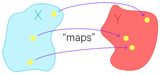
There are also values we try to predict (Y). We will use training cases to train the machine learning model so that it calculates a value for (Y), from the features in (X). Simply said, we are creating a function that operates on a set of features, (X), to produce predictions, (Y): f: X → Y.
1.1 Functions
At heart, a function is the mapping from a set in a domain to a set in a codomain. A function can map a set to itself. For example, f(x) = x2, also notated f: x ↦ x2, is the mapping of all real numbers to all real numbers, or f: R → R.
The range is the subset of the codomain which the function maps to.
Functions don’t necessarily map to every value in the codomain. Where they do, the range equals the codomain.
There are 2 sorts of functions. Functions which map to R, are known as scalar-valued or real-valued.
Functions which map to Rn where n > 1 are known as vector-valued.
Ref: Web: Mathworld Wolfram - Eric W. Weisstein.
1.2 Algorithms - Grouped by Learning Style
- Supervised learning - the algorithm is given a pre-labeled training example to learn from.
- Unsupervised learning - the algorithm is given unlabeled examples.
- Semi-supervised learning - the algorithm uses a mix of labeled & unlabeled data.
- Active learning - similar to semi-supervised learning, but the algorithm can “ask” for extra labeled data based on what it needs to improve on.
- Reinforcement learning - actions are taken and rewarded, or penalized; goal is maximizing lifetime/long-term reward (or vice versa).
Ref: Book: Neural Computing: Theory and Practice (1989) - Philip D. Wasserman.
Note: Following course guidelines, we’ll discuss the two most common methods; supervised and unsupervised.
1.3 Supervised v. Unsupervised
In a supervised learning scenario, we start with observations that include known values for the variable we want to predict. We call these labels.
Because we are starting with data that includes the label we are trying to predict, we can train the model using only some data and hold the rest for evaluating our models performance.
We’ll then use a algorithm to train a model that fits features to the known label.
As we started with a known label value, we can validate the model by comparing the value predicted by the function to the actual label value that we knew. Then, when we’re happy that the model works, we can use it with new observations for which the label is unknown, and generate new predicted values.
Typical notation:
- m = number training of examples
- x’s = input variables or features
- y’s = output variables or the “target” variable
- (x(i), y(i)) = the ith training example
- h = hypothesis i.e. the function that the algorithm learns, taking x’s as input and outputting y’s
In a unsupervised learning scenario, we don’t have any known label values in our training data set.
We’ll train the model by finding similarities between observations. Once we have trained this model, more observations are added to a cluster of observations with alike characteristics. (Cluster = Group)
2. Techniques
2.1 Regression
When we need to predict continuous valued output (i.e. a numeric value), we use a supervised learning technique called regression.
Let’s take one male. We want to model the calories burned while exercising.
First we get some pre-liminary data (age: 34, gender: 1, weight: 60, height: 165), then put him on a fitness monitor and capture additional information. Now what we do is model the calories burned using features from his exercise like his heart rate: 134, temperature: 37, and duration: 25.
In this case we know all features and have a known label value of 231 calories. So we need our algorithm to learn a function, that operates of all the males exercise features to give us a net result of 231.
f([34, 1, 60, 165, 134, 37, 25]) = 231
A sample of one person isn’t likely to give a function that generalizes well. So we gather the same data from a large number participants, and then train the model using the bigger set of data.
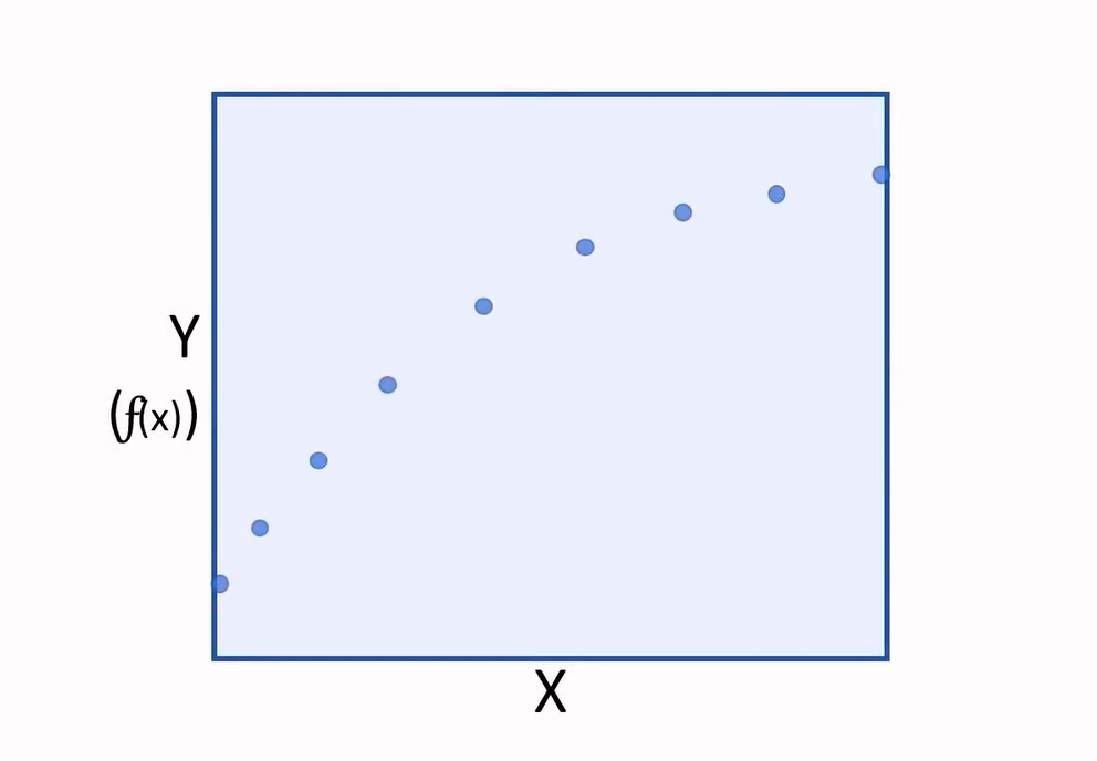
f([X1, X2, X3, X4, X5, X6, X7]) = Y
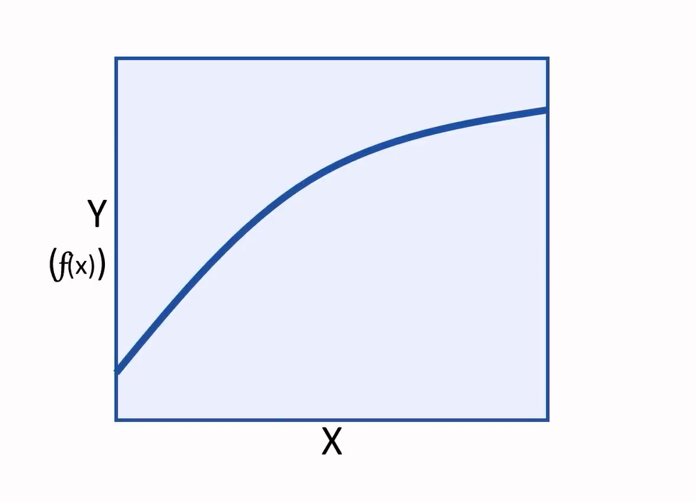
Now having a new function that can be used to calculate label (Y), we can finally plot the values of (Y) calculated for specific features of (X) values, on a chart:
And we can interpolate any new values of (X) to predict an unknown (Y).
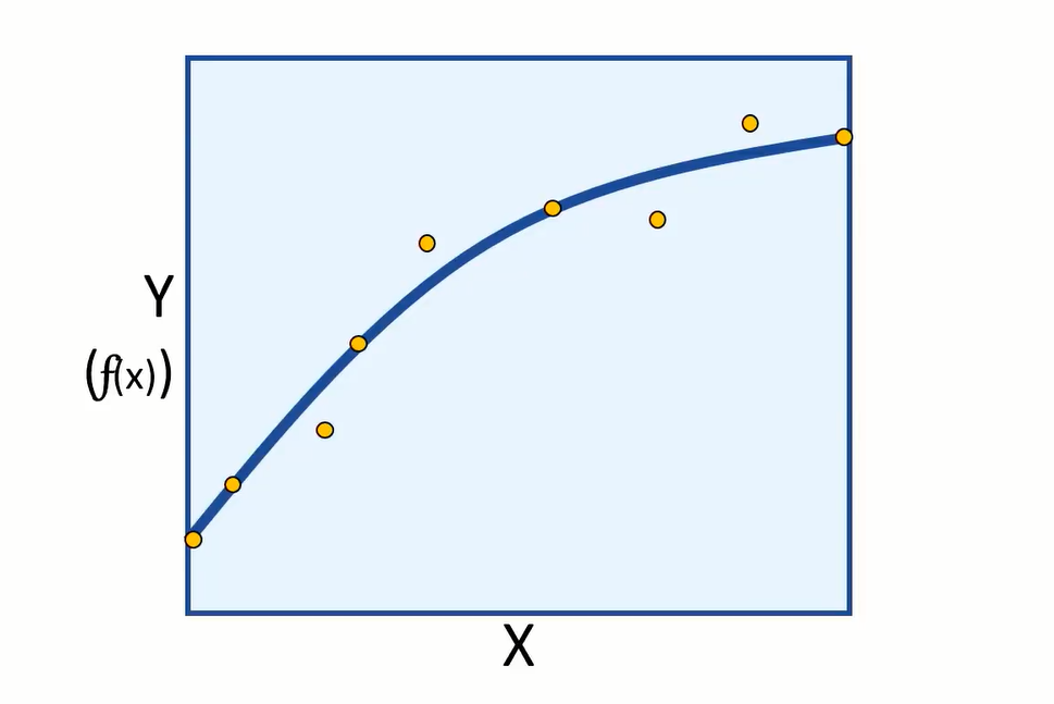
As we started with data that includes the label we try to predict, we can train the model using some data and keep the rest for evaluating the models performance. Then we can use the model to predict (F) of (X) for evaluation data, and compare the predictions or scored labels to the actual labels that we know to be true.
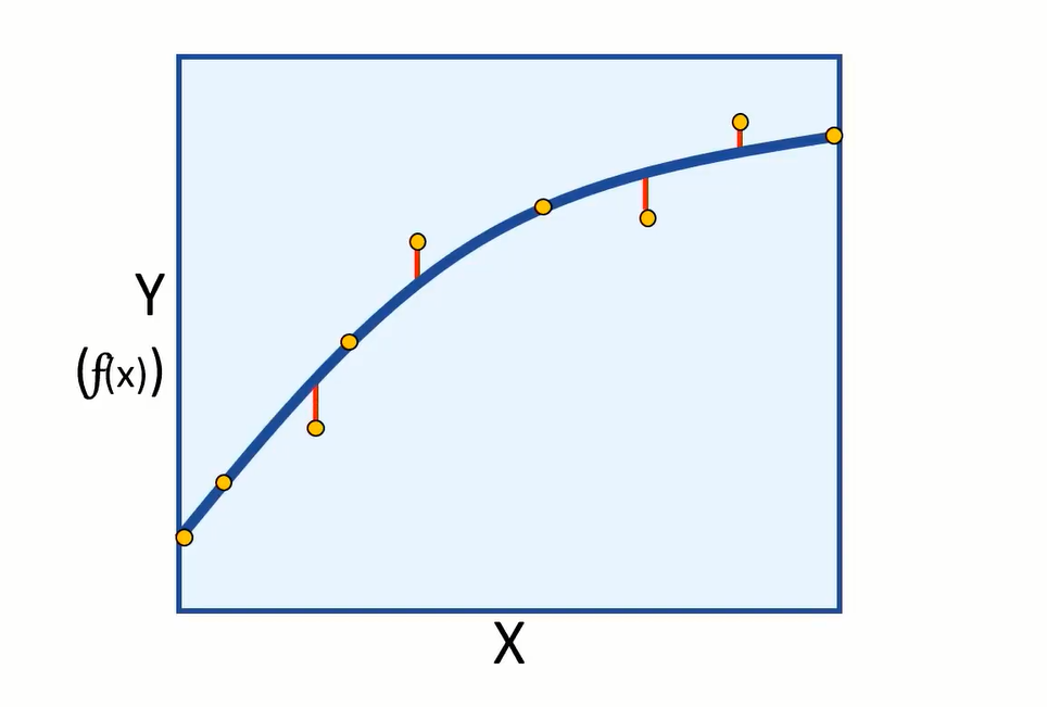
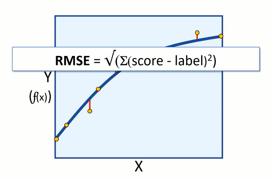
The difference between the predicted and actual levels are called the residuals. And they can tell us something about the error level in the model.
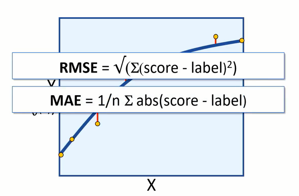
We can measure the error in the model using root-mean-square error or (RMSE) and mean absolute error (MAE).
Both are absolute measures of error in the model. For example, having an RMSE value of 5 would mean that the standard deviation of error from our test error is 5 calories. An error of 5 calories seems to indicate a reasonably good model, but let’s suppose we are predicting how long an exercise session takes. An error of 5 hours would be a very bad model.
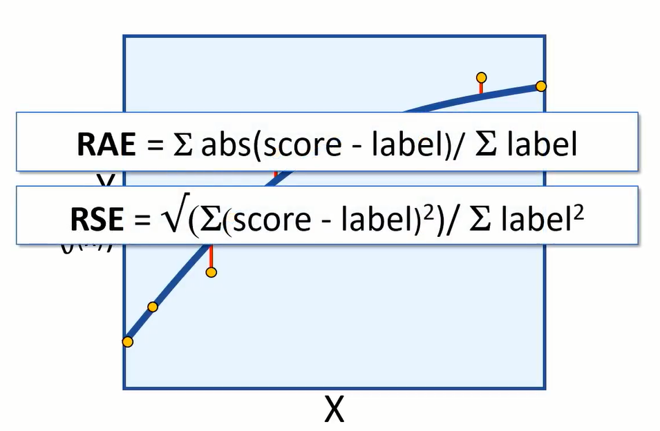
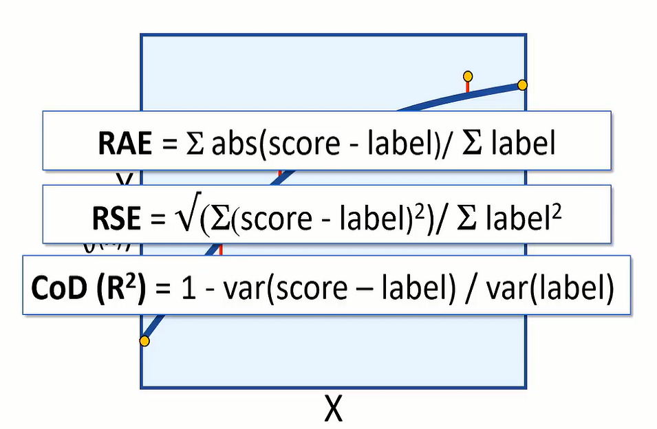
You might want to evaluate the model using relative metrics, to indicate a more general level of error as a ‘relative value’ between 0 and 1. Relative absolute error (RAE) and relative squared error (RSE) produce metrics where the closer to 0 the error, the better the model.
Coefficient of determination (CoDR) or R squared, is another relative metric, but this time a value closer to 1 indicates a good fit for the model.
2.2 Classification
Another kind of supervised learning is called classification.
Classification is the technique that we can use to predict which class or category something belongs to. A simple variant is binary classification, where we predict whether entities belong to one of two classes (true or false).
Example, we’ll take a number of patients in a health clinic, gather some personal details e.g. age: 23, pregnancy: 1, glucose: 171, BMI: 43.5, run tests, and identify which patients are diabetic and which are not.
We could learn a function that can be applied to the patient features and give us the result 1 for patients that are diabetic:
f([23, 1, 171, 43.5]) = 1
and 0 for patients that aren’t.
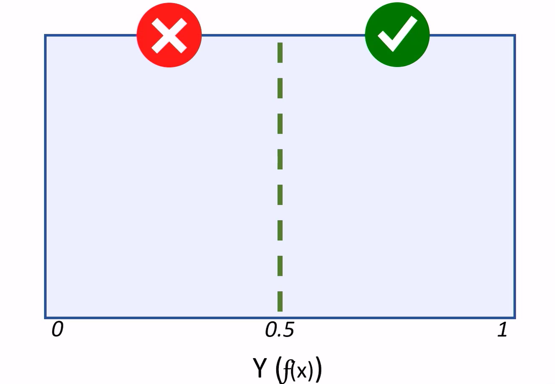
Generally, a binary classifier is a function, that can be applied to features (X), to produce a (Y) value of 1 or 0. This function won’t actually calculate the absolute value of 1 or 0. Instead it calculates a value between 1 and 0: Y(f(x)) and we’ll use a threshold value to decide whether the result should be counted as 1 or 0.
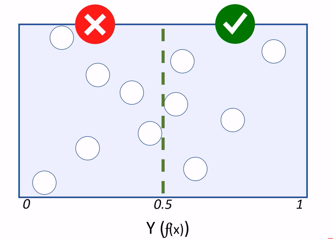
When using this model to predict values, the resulting value is classed as 1 or 0, depending on which side of the threshold line it falls.
Because classification is a supervised learning technique, we withhold some of the test data to validate the model using known labels.
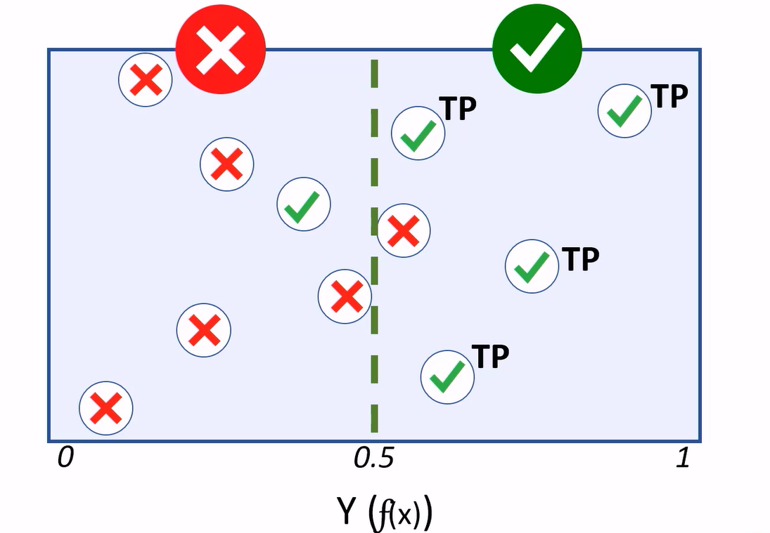
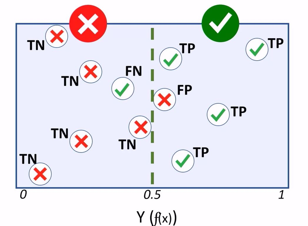
Cases where the model predicts a 1 for a test observation, while holding a label value of 1, are considered true positives.
Cases where the model predicts 0, and the actual label is 0, are true negatives.
If the model predicts 1, but the actual label is a 0, that’s a false positive.
If the model predicts 0, but the value is 1, we have a false negative.
A treshold determines how the predicted values are classified. For your diabetes model, having more false positives, thus reducing the amount of false negatives, will be better as more people with a risk of diabetes get identified.
The total number of positives and negatives generated by a model are crucial in evaluating its effectiveness. For that purpose we’ll use this confusion matrix e.g. our basis for calculating performance metrics for the classifier.
Ref: Web: MSXDAT262017 - edX.

9. In Practice
Before you start building your machine learning system, you should:
- Be explicit about the problem.
- Start with a specific question. What do you want to predict, what tools you have to predict it with?
- Brainstorm on possible strategies like what features might be useful, or do you need to collect more data?
- Try and find good input data.
- Randomly split data into: training samples, testing samples and validation samples.
- Use features of, or features built from the data, that may help with making predictions.
To start:
- Start with a simple algorithm which can be implemented quickly.
- Test the simple algorithm on your validation data, evaluate the results.
- Plot learning curves to decide where things need work. As example, do you need more data, features?
- Analysis: manually examine examples in the validation set your algorithm made errors on.
To generate a learning curve, you deliberately shrink the size of the training set and see how training and validation errors will change as you increase the size.
With smaller training sets, we expect the training error will be low because it is easier to fit to less data. As the training set size grows, your average training set error is expected to grow.
Conversely, we expect the average validation error to decrease as the training set size increases.
If the training and validation error curves flatten out at a high error as set sizes increase, then you have a high bias problem. Adding more training data will not (by itself) help much.
On the other hand, high variance problems are indicated by a large gap between training and validation error curves as training set sizes increase. You would see a low training error. In this case curves are converging and adding data helps.
Ref: Web: Intro to Artificial Intelligence - Udacity.